Project Description
In industrial environments, it is often important to be able to recognize when a machine needs to be serviced before the machine experiences a critical failure. This type of problem is often called predictive maintenance. One approach to solving predictive maintenance problems is the use of a one-class classification model for anomaly detection, where the model can make a monitoring system aware that a machine is running in a manner that is different than its standard operating behavior.
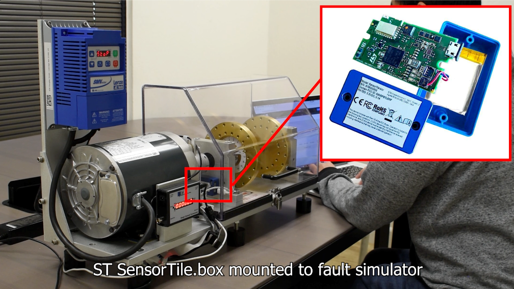
This blog describes how to use Qeexo AutoML to build a one-class classification model for anomaly detection on machine vibration data. For this application, we will be using the ST SensorTile.box, one of the many embedded hardware platforms that has been integrated into AutoML.
Problem Scenario
We will be using a fault simulator to simulate various normal or anomalous machine operating conditions. The fault simulator we are using consists of a flywheel driven by a rotational motor that can be configured to spin at various rates and can also be configured to have a number of different attachments.

Sensor Configuration
For this problem, we will select accelerometer and gyroscope sensors at an ODR of 6667 Hz, with FSRs of +/- 2g and +/- 125 dps, respectively. This should allow us to accurately capture the high frequency, high precision data typically required for machine vibration classification.

For more details about how to select an appropriate sensor configuration for any project type, check out our blog post on building Air Gesture models using Qeexo AutoML https://qeexotdkcom.wpengine.com/detecting-air-gestures-with-qeexo-automl/.
Data Collection
For this problem, we want to determine whether the machine is running normally or not. In this case, normal machine behavior is set to be approximately 1500 RPM with no physical attachments.
Since we’re going to be building a one-class, anomaly detection model, we only need to collect data under these “normal” conditions, and we will use the resulting model to determine whether or not the machine is running under these conditions.
For this case, we will collect 200 seconds of continuous “1500 RPM” data. The first 10 seconds of this data is shown in the figure below.

Model Training
After configuring our sensors and collecting our data, we are ready to build an initial model. We will select the collected data from our Training page and press “Start New Training”.
Running a benchmark build
For this demo, we’ll be testing the difference between Manual and Automatic feature selection. To start, let’s check a build with the full Qeexo AutoML feature set enabled. We’ll build a model using these features on both the accelerometer and gyroscope data. To do this, we’ll select Manual Sensor Selection on the first training settings page, and then we’ll select Manual Feature Selection on the next page, so that all of the feature groups are selected.

Next, we’ll select the maximum instance length for 6.6kHz data and a similar classification interval, 307 ms and 250 ms respectively, and we’ll select LOF model type for the build. We will use these same values for instance length, classification interval, and model type for all of the builds in this demo.

After all of the configuration parameters have been set, we can launch the build by pressing the “Start Training” button.
After training has completed, the library will be flashed to the connected device and the model results will be available on the Models tab:

As shown here, our LOF model is already able to achieve very high CV accuracy with relatively low latency and size! This suggests that this problem is solvable with Qeexo AutoML.
Running a build with Automatic Sensor & Feature Selection
Next, we’ll try running a build with Automatic Sensor & Feature Selection enabled. We’ll use most of the same settings from before, except we will select the Automatic option in the Sensor Selection pane.

Enabling this option will apply Qeexo’s selection algorithms to find the optimal sensors and features for the given problem, at the expense of increased build time. In this case, the build took about 40% longer than the all-features build.
After the build has completed, the final model will appear at the top of the Models tab:

From the image above, we can see that with AutoML’s sensor and feature selection enabled, we are able to achieve even higher model accuracy than all-features model, while also having similar latency and substantially smaller model size than the all-features model!
Finally, we will want to flash the compiled binary to our ST.box and check that the classifier is producing the expected output. As shown in the video version of this tutorial, the final model is able run inference on the embedded device and accurately recognize a variety of anomalous states, in real time. Check it out on our website at: https://qeexotdkcom.wpengine.com/video